The current forest component in FLORES includes models for growth, harvesting/utilization, and jungle rubber. It was developed by the Bukittinggi Trees & Forests Team: Ravi Prabhu, Nur Masriptin, James Gambiza, Chris Dake, Mike Spilsbury, Bruno Verbist, and Oscar García. The forest stand growth model described here benefited of inputs from all this people, although the first three and myself were more directly involved in its construction and should take the blame.
Initial discussion centered on the appropriate type of model. Individual-tree models are more intuitive and easier to build, compared with more abstract aggregated stand-level models. That level of detail, however, seemed a mismatch with the rest of FLORES. In deference to the audience, and because of limitations of time, it was also decided to use a more mechanistic approach instead of adapting an existing empirical model (e.g. [4,5]). Following Holling [3], we started looking at the outputs required by other modules, at the input information likely to be available, and tried to design the simplest model we could get away with for matching that. The result is clearly a very crude caricature of a forest. We can build arbitrarily complex models, but that was not the point. The emphasis was more on producing an appropriate FLORES module, within the time available, rather than on detailed modelling of forest development processes.
Not wishing to make it too boring though, we attempted to mimic a successional interaction of pioneer and shade-tolerant species. After bare land, pioneers come in and start growing, with tolerants establishing themselves underneath. Eventually the pioneers slow down their growth, affected by decrepitude and/or competition from the tolerants. Finally the population of pioneers crashes down and the tolerants take over. The model can be started from bare land, or used for projecting the future development of an existing forest.
In a dynamic system model, the system at any point in time is described by an appropriate set of state variables. The rate of change of these is specified by a set of differential or difference equations (transition equations), in terms of the current state and of any external control variables. Any other quantities of interest are then estimated from the state variables by output functions (see [2], for example.) The jargon tends to vary with the speaker's background:
Controls ģ inputs, policy levers, exogenous variables
State variables ģ (compartment) levels, endogenous variables
Transitions ģ flows, rates
Outputs ģ indicators
The key state variables needed to produce the required outputs were the amount per hectare of each of the two crop components, pioneers and tolerants. We initially talked about biomass, perhaps a bit self-conscious about being branded as "timber beasts". The requirements were mostly for volumes, though, so later the total stem volume per hectare was chosen. The volume of pioneers and tolerants are denoted by VP and VT, respectively.
In addition, to handle the dynamics of the system and to generate some other outputs, NP and NT kept track of the numbers of trees per hectare. A fifth state variable, the canopy top height H, was also included. In AME the state variables are represented by compartment levels, and the rates of change by flows.
The volume increment was modelled as an "assimilation" or anabolic rate, minus "overheads" or catabolic rate, minus mortality. The assimilation component represents the capture of resources per unit area in the stand. It is known that it increases as the canopy and the root system develop, reaching a roughly constant value when there is full site occupancy. This total assimilation was assumed to be shared among the trees in proportion to their individual volumes. Therefore, the assimilation for the pioneers and tolerants should be proportional to VP and VT, respectively (it may be easier to think throughout in terms of a mean tree, and multiply by N.) In order to add-up to the constant total we have to divide by VP + VT.
The less-than-full-occupancy before crown closure was modelled dividing instead by VP + VT + k, where k is some constant parameter. This is a variation on the standard rational function or hyperbola trick: The function x/(x+k) starts from zero, rising to an asymptotic value of one. The value 1/2 is reached at x = k.
The assimilation terms are then
|
The overheads/catabolic term represents losses from respiration, etc. Presumably these increase with tree size (efficiency decreases), causing the upper rounding and asymptotic trend of nice textbook sigmoids. Data from some temperate fast-growing plantations does not support this and shows no indication of curving, at least up to ages well beyond normal rotations [1], but it might be different in this situation. Besides, this is a convenient device to limit final growth for producing plausible growth trends. In particular, it makes possible to simulate the "crashing" of the pioneers that is supposed to occur at some stage.
The heroic assumption was made that this term is
|
although perhaps something proportional to N (V/N)0.5 would have been a little more logical when thinking in terms of mean trees. This particular parameterization was chosen to help in the calibration, since it can be seen that b is the asymptote that limits the maximum achievable volume (in the absence of the other crop component.)
The third term is the natural mortality in terms of volume. If mortality were the same for all tree sizes it would equal the mean tree volume times the mortality in number of trees. Because mortality tends to concentrate in the smaller trees, it was reduced by a factor of 0.75 (this has been found a reasonable approximation in pine plantations):
|
The complete volume increment equations are then:
| |||||||||||||||||||||||||||||||||||
Natural mortality is usually very erratic and difficult to estimate. There are no completely satisfactory stand-level mortality models available. To keep things simple, a constant percentage mortality rate was tried first:
| (3) |
| (4) |
For top height, the popular Richards equation was used, with a shape parameter of 0.5 in the absence of any better information:
| (5) |
The system is ruled by these equations when left to its own devices, that is, in-between management actions.
Apart from the initial number of pioneers and possibly the rate of recruitment, the controls are partial (thinning) or clear-cut harvesting actions. These usually occur at discrete points in time, causing an essentially instantaneous change of state. Therefore, perhaps it would have been more natural to implement them through jumps in the compartment levels. In AME that is a big NO-NO though, so harvesting has to be done through flows. Just keep in mind that these flows are normally step pulses at certain dates, and not continuing rates.
Four input values have to be provided: the removals of volume and number of trees per hectare for pioneers and tolerants. The relationship between volume and number may be worked out using the known average volume per tree and the nature of the harvesting action (thinning from below, etc.) The top height can be considered as unchanged by partial harvesting.
In addition to the state variables, other derived outputs may be of interest, and in fact are required by other modules. The basal areas of pioneers and tolerants, in m3/ha, are obtained from the volumes, top height, and a simple stand volume equation: V = 0.4 B H. From where,
| (6) |
The (quadratic) mean diameter, in centimeters, is computed from the basal area definition B = p/40000 D2 N:
| (7) |
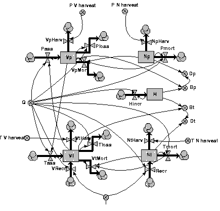
In principle, the implementation of all this in AME is straightforward (Figure 2). A possibly more elegant version, directly extendable to more than two crop components, could have used AME's multiple instances; it is left as an exercise to the reader.
A model for monospecific timber plantations could be easily derived by deleting one of the crop components (pioneers or tolerants), and choosing appropriate parameter values. Or even simpler, by setting the tolerant's recruitment to zero.
It was initially proposed to model jungle rubber cultivation systems with a relatively simple extension of the model above. The rubber trees would form part of one of the two components, with latex yields and tapping related to diameter. If really needed, a third crop component could be introduced, and a growth reduction associated with rubber tapping could be added.
Going from the differential equations to AME's discrete time formulation turned out not to be entirely trivial. AME does not currently have a numerical integration procedure for differential equations. Or, from another point of view, integrates using the so-called Euler method, a rather simplistic approach universally despised by numerical analysts.
In practice, one would expect the warnings about Euler's potential instability and other evils to be no more than scaremongering by purists and theoreticians, especially with such a ridiculously small time step, a week, relative to the time scale of forest growth processes (actually, most of the development and testing was done with 0.1 year steps, fairly small anyway.) In fact, at low state variable levels there was a disturbing tendency for things going negative, or for the system getting stuck or crashing in other ways. Nothing that could not be finally fixed by fiddling bounds and initial values, but it took a surprising amount of effort to get it right.
In particular, top height was made to start at 0.2 m, and initial and recruited trees were entered with a small non-zero volume, 0.00015 m3 (don't ask!)
Another small annoyance was AME's "feature" of refusing to take fractional powers, e . g. square roots, of zero. It was necessary to add throughout ugly conditional tests or additions of small constants to guard against error messages.
There remained the simple question of calibrating the model. Calibration, or training, are euphemisms employed by simulation modellers for the art of picking parameter values out of thin air to produce plausible behavior, as opposed to proper data-based parameter estimation.
The height submodel was easy: just choose a likely asymptote Hmax, say 40 m, and a suitable time-scaling parameter. Getting the rest of the model to behave was far from simple. Just too many interacting levers with unpredictable results, when manipulated by raw trial and error.
After many hours of frantic and unfruitful tinkering, a somewhat more structured strategy started to emerge. Try first to get sensible trends for pioneers and tolerants separately, in the absence of the other component. And concentrate in curve shapes, leaving adjusting of the time scale for later. The tolerants did fall into place relatively easily. The pioneers, however, required some rethink.
We wanted to represent a (real or imagined) build-up of pioneers biomass to a certain maximum, followed by a disintegration stage where they eventually disappear. This is quite different from typical growth models. Many of these have built-in asymptotes, but the volume never decreases. As already mentioned, even the reduction in gross volume increment seems based more on theoretical prejudice than on facts [1]. True, what goes up must come down, but: (a) managed stands are cut long before anything like that starts happening, and (b) an eventual disintegration is likely to occur through catastrophic mechanisms other than the main anabolism/catabolism/competition processes (e .g. wind, rot, etc.) The basic equations (1) and (3) are incapable of exhibiting the "crashing" behavior, and needed modification.
Incidentally, at some stage the "loss" term (VP/Vmax)1/2 had been changed to DP/Dmax, to more easily prevent the diameter from becoming ridiculously high. Anyhow, the losses can only slow down the growth rate, to reverse it it was necessary to make mortality to increase with tree size. Introducing DP as a factor in the right-hand-side of (3) did the job.
It may be mentioned that there was an attempt at adding respectability to this kludge by using instead a rather neat mortality equation (taken from an unpublished eucalypt growth model), that is compatible with the infamous -3/2 self-thinning law . The "law" essentially predicts that V/N tends asymptotically to be proportional to N-3/2. It does not work very well in practice, but it is highly praised in some circles. Unfortunately it is seen that, according to this, V could not decrease.
Having tamed the pioneers and tolerants in isolation, it remained making them to coexist. The key is the first term in the right-hand-side of (1) and (2). Essentially a partitioning coefficient of the form x/(x+y) that determines how the total gross increment is distributed among two components of sizes x and y.
As was discovered the hard way, though, this particular form of the partitioning coefficient preserves the relative sizes, not allowing the component that is behind to catch up. Either the pioneers do not take off the ground, or the tolerants can come in only after the pioneers are gone. This makes a lot of sense for monospecific cohorts, but it is not what we wanted to happen here. Presumably the tolerants are relatively more efficient at low light levels, allowing them to gain ground. A more general partitioning model for this and other situations may be based on
|
No much time for exhaustive experimentation, so we just used
|
Figure 3 shows the simulated volume of pioneers and tolerants, starting with 2000 pioneers/ha at age zero. The succession pattern seems sensible, although perhaps a narrower distance between the two peaks, and a higher degree of coexistence might have been desirable.
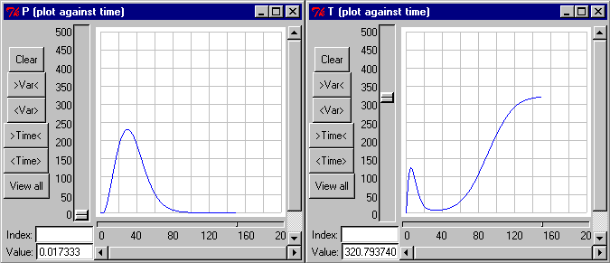
There is also an unexpected "hump" in the early development of the tolerants, before the pioneers establish themselves and take over. That this is really a glitch becomes clearer when plotting the diameters: they rise briefly to extremely high values. This was made worse by trying to suppress it through cutting down initial recruitment with the hyperbola trick, substituting
|
At the end, there was no demand from other groups for a plantation model. For rubber, there was not enough time for tuning up a modified version, so it was decided to use a different approach that had been developed independently by other team members.
The model obtained does a reasonable job of mimicking forest growth and its responses to harvesting within a FLORES prototype. Its realism could be improved with some more patient parameter tweaking (left as an exercise to the reader.)
Obviously, doing it right would be a multi-year project. The model logic seems sound, however, and something similar could form the basis for statistical parameter estimation with appropriate data.
If it becomes really necessary for the precise simulation of a wide variety of silvicultural treatments, foliage/root state variables or compartments could be added [1]. A good empirical model could also be suitable, instead of a more mechanistic one.
At any rate, it seems important to attempt the simplest possible model that adequately connects the required outputs and available inputs. Detailed process models are useful for describing and improving the understanding of systems, and it is easier to generate plausible behavior with them than with lumped or aggregated models. However, it is well-known that over-parameterization makes them less reliable for prediction purposes, apart from other disadvantages (e. g. [3], p. 50.) In principle, molecular mechanics can predict the behavior of any physical system (provided that one has a good inventory of the initial positions and velocities of all molecules.) That is nice to know, and occasionally useful. In designing a car suspension it may be more practical to use a rough empirical approximation, Newton's laws (Figure 4).